Acknowledgement

Since this is another SQL-based post, I'd like to acknowledge the massive knowledge and confidence boost I got from reading Julia Evans (aka b0rk)'s SQL zine Become a SELECT star. She has a beautiful style and breaks complex technical concepts down into easily understandable chunks with great illustrations. Reading that zine advanced my database confidence immensely.

Installing the bits you need

I assume that you've got Python installed on your system already, and that the database you want to connect to is set up and running. What you need now are the bindings for that particular database. For the Oracle database, this is a package known as cx_Oracle. For PostgreSQL, I suggest psycopg2 though there are other bindings available.

You will definitely need to install the pre-packaged database client libraries on your host (or in your container) as well. For Oracle look for your platform in the Oracle Instant Client download pages, for PostgreSQL on linux you will need libpq-dev as supplied by your package manager. On MacOS, please find the appropriate option from the PostgreSQL MacOSX download page.

After you've installed these pieces, you can then pip install --user cx_Oracle or pip install --user psycopg2. My personal preference is to install bindings in a venv. For Solaris 11 you can get the cx_Oracle bits as well as the Oracle Instant Client by uttering pkg install cx_Oracle. [On a personal note, I made that possible - see the History tab on the Solaris Userland cx_Oracle github].

Getting a connection to the database

Now that you have the correct packages installed, you can start investigating. The first thing to do is start an interactive interpreter and import the modules you need:

$ python3.8
>> import cx_Oracle

(Note that unless you're using Solaris' pre-packaged version, you must point LD_LIBRARY_PATH to where the module can locate the Instant Client libraries, specifically libclntsh.so)

$ python 3.8
>>> import psycopg2
>>> from psycopg2.extras import execute_batch

We need a connection to the database, which in Oracle terms is a DSN, or Data Source Name. This is made up of the username, password, host (either address or IP), port and database instance name. Put together, the host, port and database instance are what Oracle calls the "service name".

The common example you will see in Oracle documentation (and on stackoverflow!) is

scott/tiger@orcl:1521/orcl

I'm a bit over seeing that, so I've created a different username and DBname:

DEMOUSER/DemoDbUser1@dbhost:1521/demodb

Since Oracle defaults to using port 1521 on the host, you only need to specify the port number if your database is listening on a different port.

An Oracle connection is therefore

user = "DEMOUSER"
passwd = "DemoDbUser1"
servicename = "dbhost:1521/demodb"

try:
    connection = cx_Oracle.connect(user, passwd, servicename)
except cx_Oracle.DatabaseError as dbe:
    print("""Unable to obtain a connection to {servicename}""".format(servicename=servicename))
    raise

With PostgreSQL we can also specify whether we want SSL enabled.

try:
    connection = psycopg2.connect(dbname=dbname,
                                  user=dbuser,
                                  password=dbpassword,
                                  host=dbhost,
                                  port=dbport,
                                  sslmode=dbsslmode)
except psycopg2.OperationalError as dboe:
    print("""Unable to obtain a connection to the database.\n
          Please check your database connection details\n
          Notify dbadmin@{dbhost}""".format(dbhost=dbhost),
          file=sys.stderr, flush=True)
    raise

Once we have the connection, we need a cursor so we can execute statements:

cursor = connection.cursor()

Now that we have our connection and a cursor to use, what can we do with it? SQL baby!

We need a handy dataset to muck around with, so I've got just the thing courtesy of my previous post about determining your electorate. My JSON files have a fairly basic structure reflecting my needs for that project, but that is still sufficient our purposes here.

>>> import json
>>> actf = json.load(open("find-my-electorate/json/ACT.json", "r"))
>>> actf.keys()
dict_keys(['Brindabella', 'Ginninderra', 'Kurrajong', 'Murrumbidgee', 'Yerrabi'])
>>> actf["Yerrabi"].keys()
dict_keys(['jurisdiction', 'locality', 'blocks', 'coords'])

The 'jurisdiction' key is the state or territory name (ACT, Australian Capital Territory in this case), the 'locality' is the electorate name, 'blocks' is a list of the Australian Bureau of Statistics Mesh Block which the electorate contains, and 'coords' is a list of the latitude, longitude pairs which are the boundaries of those blocks.

Now we need a schema to operate within. This is reasonably simple - if you've done any work with SQL databases. To start with, we need two SEQUENCE s, which are database objects from which any database user may generate a unique integer. This is the easiest and cheapest way that I know of to generate values for primary key columns. (For a good explanation on them, see the Oracle 19c CREATE SEQUENCE page). After that, we'll create two tables: electorate and geopoints. (We're going to ignore the Mesh Block data, it's not useful for this example).

-- This is the Oracle DB form
DROP TABLE GEOPOINTS CASCADE CONSTRAINTS;
DROP TABLE ELECTORATES CASCADE CONSTRAINTS;

DROP SEQUENCE ELECTORATE_SEQ CASCADE;
DROP SEQUENCE LATLONG_SEQ CASCADE;

CREATE SEQUENCE ELECTORATE_SEQ INCREMENT BY 1 MINVALUE 1 NOMAXVALUE;
CREATE SEQUENCE LATLONG_SEQ INCREMENT BY 1 MINVALUE 1 NOMAXVALUE;

CREATE TABLE ELECTORATES (
    ELECTORATE_PK   NUMBER DEFAULT DEMOUSER.ELECTORATE_SEQ.NEXTVAL NOT NULL PRIMARY KEY,
    ELECTORATE      VARCHAR2(64) NOT NULL,
    STATENAME       VARCHAR2(3) NOT NULL -- Using the abbreviated form
);

CREATE TABLE GEOPOINTS (
    LATLONG_PK      NUMBER DEFAULT DEMOUSER.LATLONG_SEQ.NEXTVAL NOT NULL PRIMARY KEY,
    LATITUDE        NUMBER NOT NULL,
    LONGITUDE       NUMBER NOT NULL,
    ELECTORATE_FK   NUMBER REFERENCES ELECTORATES(ELECTORATE_PK)
);

-- Now for the PostgreSQL form
DROP TABLE IF EXISTS GEOPOINTS CASCADE;
DROP TABLE IF EXISTS ELECTORATES CASCADE;

DROP SEQUENCE IF EXISTS ELECTORATE_SEQ CASCADE;
DROP SEQUENCE IF EXISTS LATLONG_SEQ CASCADE;

CREATE SEQUENCE ELECTORATE_SEQ INCREMENT BY 1 MINVALUE 1 NO MAXVALUE;
CREATE SEQUENCE LATLONG_SEQ INCREMENT BY 1 MINVALUE 1 NO MAXVALUE;

CREATE TABLE ELECTORATES (
    ELECTORATE_PK   INTEGER DEFAULT NEXTVAL('ELECTORATE_SEQ') NOT NULL PRIMARY KEY,
    ELECTORATE      VARCHAR(64) NOT NULL,
    STATENAME       VARCHAR(3) NOT NULL -- Using the abbreviated form
);

CREATE TABLE GEOPOINTS (
    LATLONG_PK      INTEGER DEFAULT NEXTVAL('LATLONG_SEQ') NOT NULL PRIMARY KEY,
    LATITUDE        NUMERIC NOT NULL,
    LONGITUDE       NUMERIC NOT NULL,
    ELECTORATE_FK   INTEGER REFERENCES ELECTORATES(ELECTORATE_PK) NOT NULL
);

We need to execute these statements one by one, using cursor.execute(). Come back once you've done that and we've got our schema set up.

[I see that a short time has passed - welcome back]

Now we need to populate our database. For both connection types, we'll make use of prepared statements, which allow us to insert, update, delete or select many rows at a time. For the Oracle connection we'll use the executemany() function, but for PostgreSQL's psycopg2 bindings we'll use execute_batch() instead. (See the psycopg2 website note about it).

For the Oracle examples, we'll use a bind variable so that when we INSERT into the ELECTORATES table we get the ELECTORATE_PK to use in the subsequent INSERT to the GEOPOINTS table. That saves us a query to get that information. The psycopg2 module does not have this support, unfortunately. Since we have many records to process, I've created some small functions to enable DRY

# Oracle version
>>> epk = cursor.var(int)
>>> electStmt = """INSERT INTO ELECTORATES (ELECTORATE, STATENAME)
...                VALUES (:electorate, :statename)
...                RETURNING ELECTORATE_PK INTO :epk"""
>>> geoStmt = """INSERT INTO GEOPOINTS(LATITUDE, LONGITUDE, ELECTORATE_FK)
...              VALUES (:lat, :long, :fk)"""

>>> def addstate(statename):
...     for electorate in statename:
...         edict = {"electorate": statename[electorate]["locality"],
...                  "statename": statename[electorate]["jurisdiction"],
...                  "epk": epk}
...         cursor.execute(electStmt, edict)
...         points = list()
...         for latlong in statename[electorate]["coords"]:
...             points.append({"latitude": float(latlong[1]),
...                            "longitude": float(latlong[0]),
...                            "fk": int(epk.getvalue(0)[0])})
...         cursor.executemany(geoStmt, points)
...         connection.commit()

>>> allpoints = dict()
>>> states = ["act", "nsw", "nt", "qld", "sa", "tas", "wa", "vic", "federal"]

>>> for st in states:
...     allpoints[st] = json.load(open("json/{stu}.json".format(stu=st.upper()), "r"))
...     addstate(allpoints[st])

For the PostgreSQL version, we need to subtly change the INSERT statements:

>>> electStmt = """INSERT INTO ELECTORATES (ELECTORATE, STATENAME)
...                VALUES (%(electorate)s, %(statename)s)
...                RETURNING ELECTORATE_PK"""
>>> geoStmt = """INSERT INTO GEOPOINTS(LATITUDE, LONGITUDE, ELECTORATE_FK)
...                VALUES (%(latitude)s, %(longitude)s, %(fk)s)"""

Another thing we need to change is the first execute, because bind variables are an Oracle extension, and we're also going to change from executemany() to execute_batch():

>>> def addstate(statename):
...     for electorate in statename:
...         edict = {"electorate": statename[electorate]["locality"],
...                  "statename": statename[electorate]["jurisdiction"]}
...         cursor.execute(electStmt, edict)
...         epk = cursor.fetchone()[0]
...         points = list()
...         for latlong in statename[electorate]["coords"]:
...             points.append({"latitude": float(latlong[1]),
...                            "longitude": float(latlong[0]), "fk": epk})
...         execute_batch(cursor, geoStmt, points)
...         connection.commit()

The rest of the data loading is the same as with Oracle. Since I'm curious about efficiencies, I did a rough benchmark of the data load with executemany() as well, and it was around half the speed of using execute_batch(). YMMV, of course, so always test your code with your data and as close to real-world conditions as possible.

Now that we have the data loaded we can do some investigations. I'm going to show the PostgreSQL output for this and call out differences with Oracle where necessary.

While some parts of our state and territory borders follow rivers and mountain ranges, quite a lot of them follow specific latitudes and longitudes. The border between Queensland and New South Wales, for example is mostly along the 29th parallel. Between the Northern Territory and South Australia it's the 26th parallel, and that between South Australia and Western Australia is along meridian 129 East.

If you go to a mapping service and plug in 29S,141E (the line between Queensland and New South Wales):

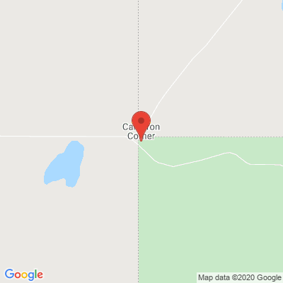
you'll see that the exact point is not where the boundary is actually drawn. That means we need to use some fuzziness in our matching.

>>> cursor.execute("""SELECT STATENAME, ELECTORATE FROM ELECTORATES E WHERE ELECTORATE_PK IN
...                   (SELECT DISTINCT ELECTORATE_FK FROM GEOPOINTS WHERE LATITUDE BETWEEN -29.001 AND -28.995)
...                   ORDER BY STATENAME, ELECTORATE""")
>>> results = cursor.fetchall()
>>> for s, e in results:
...     print("{s:6} {e}".format(s=s, e=e))
...
NSW    Ballina
NSW    Barwon
NSW    Clarence
NSW    Lismore
NSW    New England
NSW    Northern Tablelands
NSW    Page
NSW    Parkes
QLD    Maranoa
QLD    Southern Downs
QLD    Warrego
SA     Giles
SA     Grey
SA     Stuart
SA     Stuart
WA     Durack
WA     Geraldton
WA     Kalgoorlie
WA     Moore
WA     North West Central

Hmm. Not only did I not want SA or WA electorates returned, the database has also given me the federal electorates as well. Let's update our electorates table to reflect that jurisdictional issue:

>>> cursor.execute("""ALTER TABLE ELECTORATES ADD FEDERAL BOOLEAN""")
>>> connection.commit()

Popping into a psql session for a moment, let's see what we have:

demodb=> \d electorates
                                    Table "public.electorates"
    Column     |         Type          | Collation | Nullable |               Default
---------------+-----------------------+-----------+----------+-------------------------------------
 electorate_pk | integer               |           | not null | nextval('electorate_seq'::regclass)
 electorate    | character varying(64) |           | not null |
 statename     | character varying(3)  |           | not null |
 federal       | boolean               |           |          |
Indexes:
    "electorates_pkey" PRIMARY KEY, btree (electorate_pk)
Referenced by:
    TABLE "geopoints" CONSTRAINT "geopoints_electorate_fk_fkey" FOREIGN KEY (electorate_fk) REFERENCES electorates(electorate_pk)

Now let's populate that column. Unfortunately, though, some state electorates have the same name as federal electorates - and some electorate names exist in more than one state, too! (I'm looking at you, Bass!). Tempting as it is to zorch our db and start from scratch, I'm going to take advantage of this information:

1. We added the federal electorate list after all the states,

2. the federal list was constructed starting with the ACT, and therefore

3. Federal electorates will have a higher primary key value than all the states and territories.

With that in mind here's the first federal electorate entry:

demodb=> SELECT ELECTORATE_PK, ELECTORATE, STATENAME FROM ELECTORATES WHERE STATENAME = 'ACT' ORDER BY ELECTORATE_PK, STATENAME;
 electorate_pk |  electorate  | statename
---------------+--------------+-----------
             1 | Brindabella  | ACT
             2 | Ginninderra  | ACT
             3 | Kurrajong    | ACT
             4 | Murrumbidgee | ACT
             5 | Yerrabi      | ACT
           416 | Bean         | ACT
           417 | Canberra     | ACT
           418 | Fenner       | ACT
(8 rows)

Let's check how many electorates have a primary key higher than Bean:

>>> cursor.execute("""SELECT COUNT(ELECTORATE_PK), MAX(ELECTORATE_PK) FROM ELECTORATES""")
>>> cursor.fetchall()
[(566, 566)]

And a quick check to see that we do in fact have 151 electorates with that condition:

>>> 566 - 415
151

We do. Onwards.

>>> cursor.execute("""UPDATE ELECTORATES SET FEDERAL = TRUE WHERE ELECTORATE_PK > 415""")
>>> connection.commit()
>>> cursor.execute("""SELECT COUNT(*) FROM ELECTORATES WHERE FEDERAL IS TRUE""")
>>> cursor.fetchall()
[(151,)]

Likewise, we'll set the others to federal=False:

>>> cursor.execute("""UPDATE ELECTORATES SET FEDERAL = FALSE WHERE ELECTORATE_PK < 416""")
>>> connection.commit()

Back to our queries. I want to see both sorts of electorates, but grouped by whether they are federal or state electorates:

>>> cursor.execute("""SELECT E.STATENAME, E.ELECTORATE, E.FEDERAL FROM ELECTORATES E
...                   WHERE E.ELECTORATE_PK IN
...                       (SELECT DISTINCT ELECTORATE_FK FROM GEOPOINTS WHERE LATITUDE BETWEEN -29.001 AND -28.995)
...                   GROUP BY E.STATENAME, E.ELECTORATE, E.FEDERAL
...                   ORDER BY STATENAME, ELECTORATE""")
>>> fedstate = cursor.fetchall()
>>> fedstate
[('NSW', 'Ballina', False), ('NSW', 'Barwon', False), ('NSW', 'Clarence', False), ('NSW', 'Lismore', False), ('NSW', 'New England', True), ('NSW', 'Northern Tablelands', False), ('NSW', 'Page', True), ('NSW', 'Parkes', True), ('QLD', 'Maranoa', True), ('QLD', 'Southern Downs', False), ('QLD', 'Warrego', False), ('SA', 'Giles', False), ('SA', 'Grey', True), ('SA', 'Stuart', False), ('WA', 'Durack', True), ('WA', 'Geraldton', False), ('WA', 'Kalgoorlie', False), ('WA', 'Moore', False), ('WA', 'North West Central', False)]

>>> def tfy(input):
...     if input:
...         return "yes"
...     else:
...         return ""

>>> for res in fedstate:
...     fmtstr = """{statename:6} {electorate:30} {federal}"""
...     print(fmtstr.format(statename=res[0], electorate=res[1], federal=tfy(res[2])))
...
NSW    Ballina
NSW    Barwon
NSW    Clarence
NSW    Lismore
NSW    New England                    yes
NSW    Northern Tablelands
NSW    Page                           yes
NSW    Parkes                         yes
QLD    Maranoa                        yes
QLD    Southern Downs
QLD    Warrego
SA     Giles
SA     Grey                           yes
SA     Stuart
WA     Durack                         yes
WA     Geraldton
WA     Kalgoorlie
WA     Moore
WA     North West Central

I could have added a WHERE E.FEDERAL = TRUE to the query, too.

Finally, let's see what state electorates in WA and SA are on the border:

>>> cursor.execute("""SELECT STATENAME, ELECTORATE FROM ELECTORATES E
...                   WHERE ELECTORATE_PK IN
...                       (SELECT DISTINCT ELECTORATE_FK FROM GEOPOINTS WHERE LATITUDE BETWEEN -60.00 AND -25.995
                           AND LONGITUDE BETWEEN 128.995 AND 129.1)
...                   AND FEDERAL = FALSE ORDER BY STATENAME, ELECTORATE""")
>>> results = cursor.fetchall()
>>> for _res in results:
...     print("""{statename:6} {electorate}""".format(statename=_res[0], electorate=_res[1]))
...
NT     Namatjira
SA     Giles
WA     Kalgoorlie
WA     North West Central

Why do we have that electorate from the Northern Territory? It's because the coordinates are a bit fuzzy and we had to use a range (the BETWEEN) in our query.

Finally

I apologise, because while this was supposed to be a brief introduction I did get side-tracked with data investigation. I suppose that's an occupational hazard since I'm a Data Engineer working for a company which provides GIS-related services. Anyway, in terms of depth, this was definitely only scratching the surface of what is possible with Python and databases. I encourage you to go and read the Python Database API as well as the SQL reference manual(s) for your chosen database and its binding documentation.